Fitting Distribution Families with famish • famish

famish works with distribution families—sets of related distributions indexed by parameters—rather than single distributions. For example, the Normal family is indexed by its mean and standard deviation, while the Beta family is indexed by shape parameters $\alpha$ and $\beta$ . Once parameters are fixed, you have a specific distribution inside the family.

famish aims to connects those families to data (or other targets such as expert-elicited quantiles) using two ideas:

Fitting narrows a family to a single distribution. This is the functionality provided today via fit_dst() and the fit_dst_*() wrappers.
Refining narrows a family to a smaller sub-family that satisfies constraints. This capability is on the roadmap but not yet implemented.

Because fitting must return a single distribution, failure handling matters. You control this via the on_unres argument: return a Null distribution (default) or raise an error.

A quick fitting workflow

Start by loading famish and the core probaverse package, distionary. In practice, you will most likely just load the whole probaverse with library(probaverse) instead.

library(distionary)
library(famish)

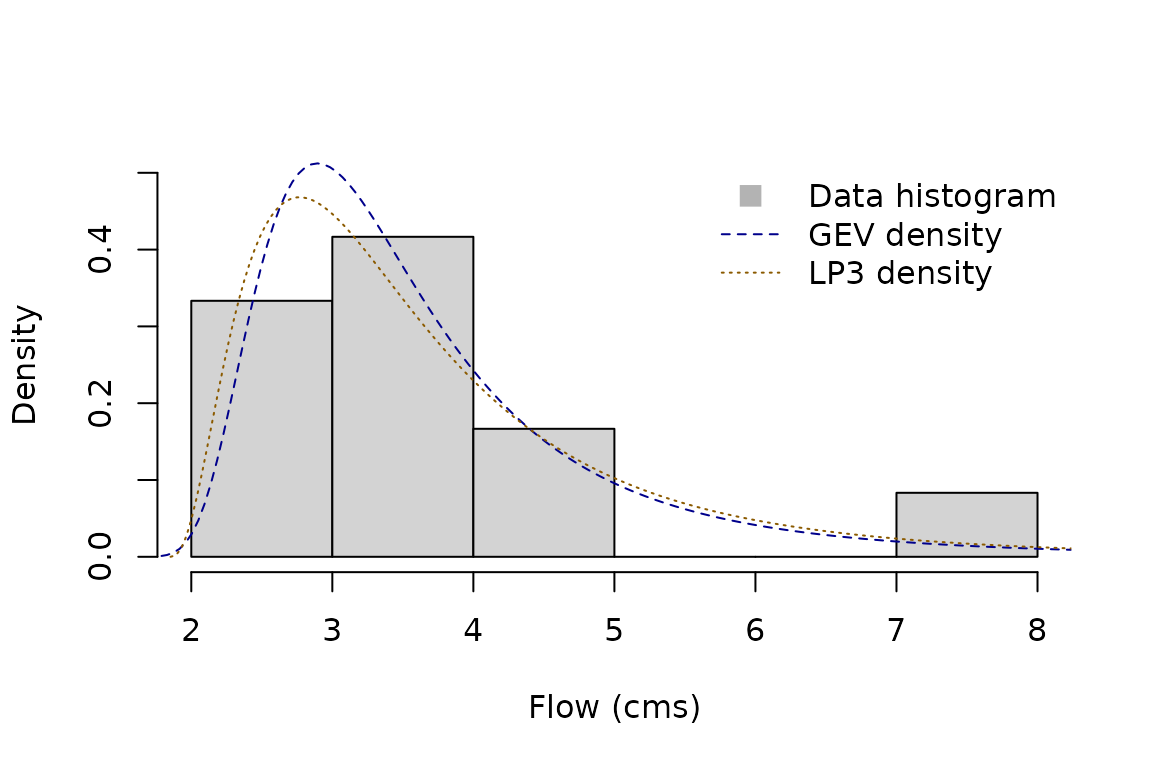
Suppose we have annual streamflow maxima (cubic meters per second) for 12 years. We will fit two distributions from two different families.

x <- c(4.0, 2.7, 3.5, 3.2, 7.1, 3.1, 2.5, 5.0, 2.3, 4.5, 3.0, 3.8)

Fit a Generalised Extreme Value (GEV) distribution with maximum-likelihood estimation using its wrapper:

gev <- fit_dst_gev(x)
#> Loading required namespace: testthat
gev
#> Generalised Extreme Value distribution (continuous) 
#> --Parameters--
#>  location     scale     shape 
#> 3.0658476 0.7426435 0.2699160

You can also call fit_dst() directly to use other combinations. Here we fit a Log Pearson Type III distribution using L-moments on the log scale:

lp3 <- fit_dst("lp3", x, method = "lmom-log")
lp3
#> Log Pearson Type III distribution (continuous) 
#> --Parameters--
#>   meanlog     sdlog      skew 
#> 1.2652738 0.3382651 1.0430967

Both fits return distionary objects, so any downstream probaverse tooling applies. Basic comparisons start with visual diagnostics:

hist(x, freq = FALSE, ylim = c(0, 0.5), main = NULL, xlab = "Flow (cms)")
plot(gev, "density", add = TRUE, n = 400, lty = 2, col = "blue4")
plot(lp3, "density", add = TRUE, n = 400, lty = 3, col = "orange4")
legend(
  "topright",
  legend = c("Data histogram", "GEV density", "LP3 density"),
  lty = c(NA, 2, 3),
  pch = c(15, NA, NA),
  col = c("gray70", "blue4", "orange4"),
  pt.cex = c(1.5, NA, NA),
  bty = "n"
)

Diagnostics that emphasise extremes

Risk-focused work often requires tail checks. famish exposes empirical ranking and quantile scores so you can benchmark fitted models.

Return levels at common periods (2-, 5-, 10-, 20-, 50-, 100-, 200-year) provide one view:

quantiles <- enframe_return(
  gev, lp3,
  at = c(2, 5, 10, 20, 50, 100, 200),
  arg_name = "return_period",
  fn_prefix = "flow"
)
quantiles
#> # A tibble: 7 × 3
#>   return_period flow_gev flow_lp3
#>           <dbl>    <dbl>    <dbl>
#> 1             2     3.35     3.35
#> 2             5     4.44     4.57
#> 3            10     5.37     5.58
#> 4            20     6.45     6.70
#> 5            50     8.20     8.43
#> 6           100     9.84     9.95
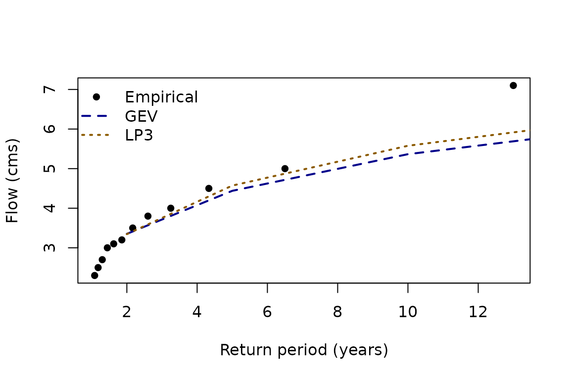
#> 7           200    11.8     11.7

Plotting the empirical data against fitted curves highlights tail behaviour.

x_return_periods <- rpscore(x, pos = "Weibull")

plot(
  sort(x_return_periods), sort(x),
  xlab = "Return period (years)",
  ylab = "Flow (cms)",
  pch = 16, col = "black"
)
lines(quantiles$return_period, quantiles$flow_gev, col = "blue4", lty = 2, lwd = 2)
lines(quantiles$return_period, quantiles$flow_lp3, col = "orange4", lty = 3, lwd = 2)
legend(
  "topleft",
  legend = c("Empirical", "GEV", "LP3"),
  col = c("black", "blue4", "orange4"),
  pch = c(16, NA, NA),
  lty = c(NA, 2, 3),
  lwd = 2,
  bty = "n"
)

Quantile scores provide a quantitative metric for how well a quantile is estimated. Lower scores indicate better calibration at the specified quantile level (Gneiting, 2011).

gev_100y <- quantiles$flow_gev[quantiles$return_period == 100]
lp3_100y <- quantiles$flow_lp3[quantiles$return_period == 100]

qs_gev <- quantile_score(x, gev_100y, tau = 1 - 1 / 100)
qs_lp3 <- quantile_score(x, lp3_100y, tau = 1 - 1 / 100)

c(GEV = mean(qs_gev), LP3 = mean(qs_lp3))
#>        GEV        LP3 
#> 0.06112929 0.06220155

Supported methods and failure handling

fit_dst() dispatches to different estimation routines:

lmom and lmom-log use the lmom package (or internal implementations for simple families).
mle uses ismev for the GEV, GP, and Gumbel families; otherwise it falls back to fitdistrplus.
Other supported methods (mge, mme) are routed through fitdistrplus.

Wrappers such as fit_dst_gev() or fit_dst_norm() document the combinations that have been verified by extensive testing. Unsupported combinations trigger a warning and still attempt fitting through fitdistrplus.

Failure can happen when data are incompatible with a distribution (e.g., negative observations for an exponential fit) or when the combination is not yet implemented. You can control the failure behaviour via:

na_action: how missing values are handled ("null", "drop", or "fail").
on_unres: what to do when a distribution cannot be resolved ("null" or "fail").

Roadmap

Current development focuses on fitting. Future releases aim to:

add “refining” tools that keep families but impose constraints (e.g., matching moments),
expose more control over underlying estimation routines,
expand diagnostics tailored to extreme-value analysis.

References

Gneiting, T. (2011). Making and evaluating point forecasts. Journal of the American Statistical Association, 106(494), 746–762.